Pandista: Panel data in discrete-time state models

Pandista is an R package that fits parameterized state models to panel (longitudinal) event data, where an individual subject’s events are known to occur at exact discrete timepoints, and such timepoints are common across the entire sample of subjects. Transition probabilities are modelled via multinomial logistical regression, allowing both static and time-varying covariates within each subject. Both continuous and categorical covariates may be used. The regression constant terms are treated as time-dependent quantities that can be specified in an arbitrary piecewise manner for each transition to establish a “baseline effect” functions which is then modified by the individual covariates. Maximum likelihood calculations are carried out in C++, and standard errors for model parameters are calculated using the numerically estimated Hessian. Uncertainty intervals for marginal state probabilities (including group differences) are estimated by Monte Carlo resampling.

Details

Transient and terminal states

Consider a five-state model in which all subjects begin in State 1, and can transition to States 2 or 3. Subjects who transition to State 3 can further transition to States 4 or 5. Graphically, the state model is:

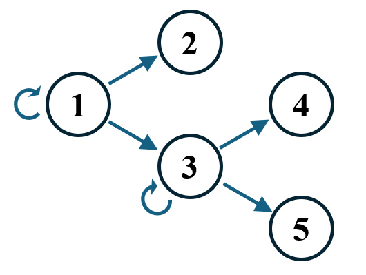
Each arrow in the diagram is a unique transition. Note that States 1 and 3 have “loop” arrows; as it customary for discrete-time state models, the subject may remain in their current state at any timepoint; we generically refer to these events as ‘transitions’ too, even though the state value is not changing. States 1 and 3 are referred to as transient states, as they have paths leading out of them to other states. States 2, 4, and 5 are referred to as terminal states; once a subject is in a terminal state, no further change in state can take place. (Technically, we could draw loop arrows on the terminal states as well, to emphasize that remaining is the only transition allowed, with probability 1; however as is custom we omit these arrows.)

Transition probabilities

A core concept in this approach is that we model the transitions between states, not the states themselves. So, for example, if a subject is in State 1 at time n, and then in State 2 at time n+1, the regressions functions model the transition probability P(1 -> 2). If that subject were still in State 1 at time n+1 (that is, no change in state took place), then the regression functions model the transition probability P(1 -> 1). The covariate values used in the regression functions for the transition from time n to time n+1 are those that exist at time n.

As a consequence, the data supplied to pandista must have a row for each timepoint for each subject, and each row will have a “from” state value and a “to” state value, representing the transition “from -> to”. All timepoints must be represented for each subject, but only up to the time at which the subject transitions to a terminal state (after which time the probability is unity that the subject will remain in that terminal state, and thus there is nothing to model).

Block decomposition

Pandista can handle state models with an arbitrary number of states and an arbitrary number of connections between those states (ie, a general Markov model). From each transient state, the total probability of the transitions leading out of that state (including the probability of remaining in state) must sum to 1 at every timepoint. However, each transient state is handled independently, that is, the probability of leaving one transient state is independent of the probability of leaving a different transient state. Therefore we may fit each transient state’s associated transition probabilities as a single block. If there is more than one block, each block is fit independently and separately from the other blocks, using only those rows from the panel data that pertain to the transitions in that block.

In the example above, we have two blocks, defined by the two transient states, State 1 and State 3; the blocks can be visualized as two separate models:

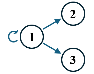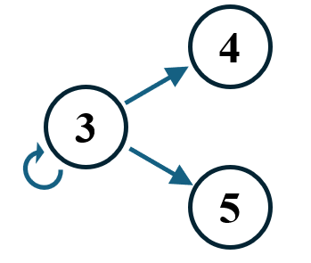Each block constitutes a single instance of a multinomial logistic regression model in which the outcome is one of the possible transitions within that block.

Time effects as intercept coefficients

The underlying probabilities for the multinomial logistic regression are specified for the $i^{th}$ event and the $k^{th}$ transition as

$P(i,k) = \frac{e^{\beta_k X_i + \alpha_k(t_i)}}{1 + \displaystyle\sum_{k \neq K}e^{\beta_k X_i + \alpha_k(t_i)}}$

where $X_i$ is the vector of covariate values associated with the $i^{th}$ event, and $\beta_k$ is the vector of coefficients associated with the $k^{th}$ transition. $K$ is the arbitrarily-chosen “reference category”, and we have

$P(i,K) = \frac{1}{1 + \displaystyle\sum_{k \neq K}e^{\beta_k X_i + \alpha_k(t_i)}}$

so that for each event $i$ we satisfy $\displaystyle\sum_k P(i,k) = 1$

Normally, the constant (intercept) terms in regression equations are absorbed into the covariates for notational convenience; here we separate them out and allow them to vary as functions of (discrete) time. For the $i^{th}$ event occurring at timepoint $t_i$ , we use $\alpha_k(t_i)$ as the intercept term in $k^{th}$ transition probability.

Accordingly, since we have a common set of $n$ sequential timepoints $1, 2, \ldots, n$ across all events in the study, the actual intercept coefficients to be estimated are the values $\alpha_k(1), \alpha_k(2), \ldots, \alpha_k(n)$ . If they are all uniquely specified, we have $(K-1)n$ of them to estimate. Because this may lead to a large number of coefficients, some of which may have high estimation uncertainty, we can “couple” two or more intercept coefficients by allowing the introduction of constraints of the form $\alpha_k(T_a + 1) = \alpha_k(T_a)$ where the pair of timepoints $T_a + 1$ and $T_a$ are consecutive values in the timepoint sequence, and a single coefficient represents both intercepts. We can extend this arbitrarily, eg, $\alpha_k(T_a + 2) = \alpha_k(T_a + 1) = \alpha_k(T_a)$ , leading us to a “changepoint model” for the intercept coefficients.

Example

Here is a simple simulated dataset containing 4766 subjects with two continuous-valued covariates “x1” and “x2”, a binary covariates “x3”, and a four-level categorical covariate “x4”. The state model is a simple single-block design with initial state 1 leading to terminal states 2 and 4. There are 15 timepoints.

load(url("http://pandista.rovero.org/data/test_df.dat"))
head(df)
#>   id t from to        x1       x2 x3 x4
#> 1  1 1    1  1 0.7773828 1.198902  1  4
#> 2  1 2    1  1 0.7773828 1.198902  1  4
#> 3  1 3    1  1 0.7773828 1.198902  1  4
#> 4  1 4    1  1 0.7773828 1.198902  1  4
#> 5  1 5    1  1 0.7773828 1.198902  1  4
#> 6  1 6    1  1 0.7773828 1.198902  1  4
table(df$t)
#> 
#>    1    2    3    4    5    6    7    8    9   10   11   12   13   14   15 
#> 4766 3745 2901 2292 1799 1368 1081  828  653  510  393  303  237  184  140

We first declare the continuous and categorical covariates. We also choose transition 1->1 as the “reference” transition:

  cov.c <- c("x1", "x2")
  cov.i <- c("x3", "x4")
  
  bt1 <- c("1->1")

We then choose changepoints for the dynamic intercept model (t=1 and t=5 for the transition 1->2, and t=1, t=6, and t=12 for the transition 1->4):


  cp1 <- list()
  cp1[["1->2"]] <- c(1, 5)
  cp1[["1->4"]] <- c(1, 6, 12)

To fit the model, we issue the call

library(pandista)
#> -----------------------------------------
#> This is pandista!
#> 
#> The package is in development.
#> Please visit pandista.rovero.org for
#> developer contact info.
#> -----------------------------------------
results <- pandista(df, i.covlist = cov.i, c.covlist = cov.c, changePointsList = cp1, basetrans = bt1)
#> Number of unique IDs: 4766 
#> 
#> Raw counts of all transition events:
#> (rows are 'from state', columns are 'to state')
#>    
#>         1     2     4
#>   1 17333   659  3208
#> 
#> 
#> Covariate list: x1 x2 x3 x4_2 x4_3 x4_4 
#> 
#> Option:  time.as.delta =  FALSE 
#> 
#> Number of blocks: 1 
#> 
#> ------------------
#> Processing block #1
#> ------------------
#> Mapped time constants with event counts:
#> 
#>       t.event
#> label     1    5    6   12
#>   1->2  407  252    0    0
#>   1->4 2365    0  707  136
#> 
#> There are 17 total coefficients to estimate for block 1 .
#> 
#> Fitting block #1
#> Using C++ code for likelihood ...
#> Calling optim ...
#> initial  value 23.290581 
#> iter  10 value 11.879782
#> iter  20 value 11.819346
#> iter  30 value 11.814001
#> final  value 11.813961 
#> converged
#> Estimating Hessian ...
#> Hessian is full rank.
#> Fit statistics for block 1:
#> AIC =  23661.9218743798 
#> Log-Likelihood =  11813.9609371899 
#> 
#> Total Log-Likelihood =  11813.9609371899

We can view the estimated coefficients in a simple table format with

table.model.coeffs(results)
#>    block block.pos trans covariate time_flag ordered.pos     est_beta
#> 3      1         1  1->2        x1         0           3 -0.187052429
#> 4      1         2  1->2        x2         0           4  0.060925711
#> 5      1         3  1->2        x3         0           5 -0.032455539
#> 6      1         4  1->2      x4_2         0           6  0.142653611
#> 7      1         5  1->2      x4_3         0           7 -0.086824059
#> 8      1         6  1->2      x4_4         0           8 -0.167931296
#> 1      1         7  1->2       t.1         1           1 -3.207857498
#> 2      1         8  1->2       t.5         1           2 -3.087815577
#> 12     1         9  1->4        x1         0          12  0.001399200
#> 13     1        10  1->4        x2         0          13  0.026686874
#> 14     1        11  1->4        x3         0          14  0.005268363
#> 15     1        12  1->4      x4_2         0          15  0.108213455
#> 16     1        13  1->4      x4_3         0          16  0.181303480
#> 17     1        14  1->4      x4_4         0          17  0.283634998
#> 9      1        15  1->4       t.1         1           9 -1.909525673
#> 10     1        16  1->4       t.6         1          10 -1.948947855
#> 11     1        17  1->4      t.12         1          11 -1.850459053
#>        est_se         LCL         UCL          pval sig
#> 3  0.13629129 -0.41123165  0.03712679  1.699246e-01    
#> 4  0.07867540 -0.06848380  0.19033522  4.386982e-01    
#> 5  0.08130876 -0.16619655  0.10128548  6.897723e-01    
#> 6  0.13818885 -0.08464681  0.36995404  3.019273e-01    
#> 7  0.14403522 -0.32374092  0.15009280  5.466435e-01    
#> 8  0.12786155 -0.37824483  0.04238224  1.890536e-01    
#> 1  0.16174394 -3.47390261 -2.94181239  1.547338e-87  **
#> 2  0.16515382 -3.35946943 -2.81616172  5.275948e-78  **
#> 12 0.06604211 -0.10723040  0.11002880  9.830969e-01    
#> 13 0.03809307 -0.03597066  0.08934441  4.835713e-01    
#> 14 0.03924984 -0.05929187  0.06982860  8.932236e-01    
#> 15 0.07570018 -0.01630227  0.23272918  1.528604e-01    
#> 16 0.07497902  0.05797396  0.30463300  1.560368e-02  **
#> 17 0.06690426  0.17358728  0.39368272  2.241022e-05  **
#> 9  0.08284916 -2.04580041 -1.77325093 1.532617e-117  **
#> 10 0.08892453 -2.09521569 -1.80268002 1.793544e-106  **
#> 11 0.12174326 -2.05070890 -1.65020920  3.553352e-52  **

Installation in R

This package is in the development stage! Feedback and questions are welcome.

Code is available at https://github.com/robert-rovetti/pandista. You can install the development version of pandista in R by running:

library(pak)
pak("robert-rovetti/pandista")